

GetTDDataInformation regarding prices and yields of bonds issued by the Brazilian government can be downloaded manually as excel files from the Tesouro Direto website. However, it is painful to aggregate all of this data into something useful as the several files don’t have an uniform format.
Package GetTDData makes the process of importing data
from Tesouro direto much easier. All that you need in order to download
the data is the name of the assets (LFT, LTN, NTN-C, NTN-B, NTN-B
Principal, NTN-F).
# from CRAN (stable version)
install.package('GetTDData')

# from github (development version)
devtools::install_github('msperlin/GetTDData')Suppose you need financial data (prices and yields) for a bond of type LTN with a maturity (end of contract) at 2023-01-01. This bullet bond is the most basic debt contract the Brazilian government issues. It does not pay any value (coupon) during its lifetime and will pay 1000 R$ at maturity.
In order to get the data, all you need to do is to run the following code in R:
library(GetTDData)

assets <- 'LTN'   # Identifier of assets
first_year <- 2020
last_year <- 2022

df_td <- td_get(assets,
                first_year,
                last_year)
#>
#> ── Downloading TD files
#> ℹ Downloading 3 files in parallel...
#> ✔ All downloads completed successfully.
#>
#> ── Checking files
#> ✔ Found 3 files
#>
#> ── Reading files
Let’s plot the prices to check if the code worked:
library(ggplot2)
library(dplyr)
#>
#> Attaching package: 'dplyr'
#> The following objects are masked from 'package:stats':
#>
#>     filter, lag
#> The following objects are masked from 'package:base':
#>
#>     intersect, setdiff, setequal, union

# filter  LTN
my_asset_code <- "LTN 010123"

LTN <- df_td %>%
  filter(asset_code  ==  my_asset_code)

p <- ggplot(data = LTN,
            aes(x = as.Date(ref_date),
                y = price_bid,
                color = asset_code)) +
  geom_line(linewidth = 1) + scale_x_date() + labs(title = '', x = 'Dates')

print(p)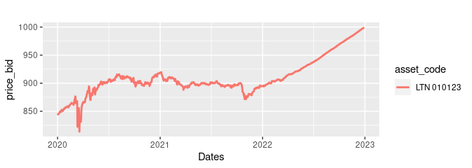
The latest version of GetTDData offers function
get_yield_curve to download the current Brazilian yield
curve directly from Anbima. The yield curve is a tool of financial
analysts that show, based on current prices of fixed income instruments,
how the market perceives the future real, nominal and inflation returns.
You can find more details regarding the use and definition of a yield
curve in [Investopedia][https://www.investopedia.com/terms/y/yieldcurve.asp].
df_yield <- get_yield_curve()
str(df_yield)
And we can plot it for the desired result:
library(ggplot2)

p <- ggplot(df_yield, aes(x=ref_date, y = value) ) +
  geom_line(size=1) + geom_point() + facet_grid(~type, scales = 'free') +
  labs(title = paste0('The current Brazilian Yield Curve '),
       subtitle = paste0('Date: ', df_yield$current_date[1]))

print(p)